This Jupyter notebook can be downloaded from check_phase_connection.ipynb, or viewed as a python script at check_phase_connection.py.

Check for phase connection

This notebook is meant to answer a common type of question: when I have a solution for a pulsar that goes from \({\rm MJD}_1\) to \({\rm MJD}_2\), can I confidently phase connect it to other data starting at \({\rm MJD}_3\)? What is the phase uncertainty bridging the gap from \(\Delta t={\rm MJD}_3-{\rm MJD}_2\)?

This notebook will start with standard pulsar timing. It will then use the simulation/calculate_random_models function to propagate the phase uncertainties forward and examine what happens.

import matplotlib.pyplot as plt
import numpy as np
import astropy.units as u

import pint.fitter, pint.toa, pint.simulation
from pint.models import get_model_and_toas
from pint import simulation
import pint.config
import pint.logging

# setup logging
pint.logging.setup(level="INFO")

1

# use the same data as `time_a_pulsar` notebook
parfile = pint.config.examplefile("NGC6440E.par")
timfile = pint.config.examplefile("NGC6440E.tim")

# we will do this very simply - ignoring some of the TOA filtering
m, t = get_model_and_toas(parfile, timfile)
f = pint.fitter.WLSFitter(t, m)
f.fit_toas()

INFO     (pint.observatory              ): Applying GPS to UTC clock correction (~few nanoseconds)
INFO     (pint.observatory              ): Using global clock file for gps2utc.clk with bogus_last_correction=False
INFO     (pint.observatory              ): Applying TT(TAI) to TT(BIPM2019) clock correction (~27 us)
INFO     (pint.observatory              ): Loading BIPM clock version bipm2019
INFO     (pint.observatory.global_clock_corrections): File T2runtime/clock/tai2tt_bipm2019.clk to be downloaded due to download policy if_missing: https://raw.githubusercontent.com/ipta/pulsar-clock-corrections/main/T2runtime/clock/tai2tt_bipm2019.clk
INFO     (pint.observatory              ): Using global clock file for tai2tt_bipm2019.clk with bogus_last_correction=True
INFO     (pint.observatory.clock_file   ): Disregarding suspicious MJD -2271.5 in TEMPO clock file
INFO     (pint.observatory              ): Using global clock file for time_gbt.dat with bogus_last_correction=False
INFO     (pint.observatory.topo_obs     ): Applying observatory clock corrections for observatory='gbt'.
INFO     (pint.solar_system_ephemerides ): Set solar system ephemeris to de421 from download
INFO     (pint.observatory              ): Applying TT(TAI) to TT(BIPM2023) clock correction (~27 us)
INFO     (pint.observatory              ): Loading BIPM clock version bipm2023
INFO     (pint.observatory              ): Using global clock file for tai2tt_bipm2023.clk with bogus_last_correction=False

np.longdouble('59.57471349427808678')

print("Current free parameters: ", f.model.free_params)

Current free parameters:  ['RAJ', 'DECJ', 'F0', 'F1', 'DM']

print(f"Current last TOA: MJD {f.model.FINISH.quantity}")

Current last TOA: MJD 54187.58732417023

# pretend we have new observations starting at MJD 59000
# we don't need to track things continuously over that gap, but it helps us visualize what's happening
# so make fake TOAs to cover the gap
MJDmax = 59000
# the number of TOAs is arbitrary since it's mostly for visualization
tnew = pint.simulation.make_fake_toas_uniform(f.model.FINISH.value, MJDmax, 50, f.model)

INFO     (pint.simulation               ): Using CLOCK = BIPM2019 from the given model

# make fake models crossing from the last existing TOA to the start of new observations
dphase, mrand = simulation.calculate_random_models(f, tnew, Nmodels=100)
# this is the difference in time across the gap
dt = tnew.get_mjds() - f.model.PEPOCH.value * u.d

Compare against an analytic prediction which focused on the uncertainties from \(F_0\) and \(F_1 = \dot F\):

\[\Delta \phi^2 = (\sigma_{F0} \Delta t)^2 + (0.5 \sigma_{F1} \Delta t^2)^2\]

where \(\Delta t\) is the gap over which we are extrapolating the solution.

analytic = np.sqrt(
    (f.model.F0.uncertainty * dt) ** 2 + (0.5 * f.model.F1.uncertainty * dt**2) ** 2
).decompose()

plt.plot(tnew.get_mjds(), dphase.std(axis=0), label="All Free")
tnew.get_mjds() - f.model.PEPOCH.value * u.d
plt.plot(tnew.get_mjds(), analytic, label="Analytic")
plt.xlabel("MJD")
plt.ylabel("Phase Uncertainty (cycles)")
plt.legend()

<matplotlib.legend.Legend at 0x74abca1ee7d0>

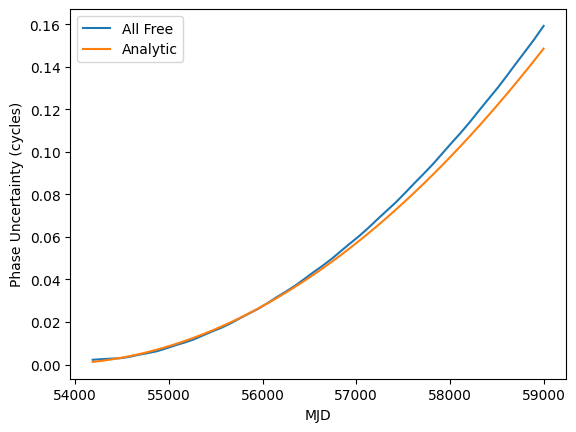
You can see that the max uncertainty is about 0.14 cycles. So that means that even at \(3\sigma\) confidence, we can be sure that we will have \(<1\) cycle uncertainty in extrapolating from the end of the existing solution to MJD 59000. The analytic solution has the same shape as the numerical solution although it is slightly lower, which makes sense since the analytic solution ignores the covariance between \(F_0\) and \(F_1\), plus uncertainties on the other free parameters (\(\alpha\), \(\delta\), \({\rm DM}\)).