This Jupyter notebook can be downloaded from solar_wind.ipynb, or viewed as a python script at solar_wind.py.
Solar Wind Models
The standard solar wind model in PINT is implemented as the NE_SW parameter (Edwards et al. (2006)), which is the solar wind electron density at 1 AU (in cm\(^{-3}\)). This assumes that the electron density falls as \(r^{-2}\) away from the Sun. With SWM=0 this is all that is allowed.
However, in You et al. (2007) and You et al. (2012), they extend the model to other radial power-law indices \(r^{-p}\) (also see Hazboun et al. (2022)). This is now implemented with SWM=1 in PINT (and the power-law index is SWP).
Finally, it is clear that the solar wind model can vary from year to year (or even over shorter timescales). Therefore we now have a new SWX model (like DMX) that implements a separate solar wind model over different time intervals.
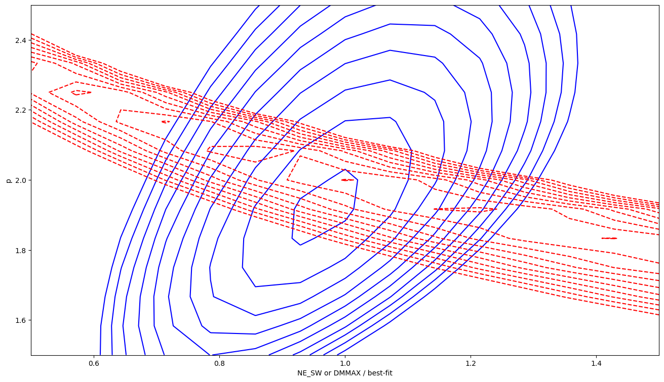
With the new model, though, there is covariance between the power-law index SWP and NE_SW, since most of the fit is determined by the maximum excess DM in the data. Therefore for the SWX model we have reparameterized it to use SWXDM: the max DM at conjunction. This makes the covariance a lot less. And to ensure continuity, this is explicitly the excess DM, so the DM from the SWX model at opposition is 0.
[1]:
from io import StringIO
import numpy as np

from astropy.time import Time
import astropy.coordinates
from pint.models import get_model
from pint.fitter import Fitter
from pint.simulation import make_fake_toas_uniform
import pint.utils
import pint.gridutils
import pint.logging

import matplotlib.pyplot as plt

pint.logging.setup(level="WARNING")
[1]:
1
Demonstrate the change in covariance going from NE_SW to DMMAX
[2]:
par = """
PSR J1234+5678
F0 1
DM 10
ELAT 3
ELONG 0
PEPOCH 54000
EPHEM DE440
"""
[3]:
# basic model using standard SW
model0 = get_model(StringIO("\n".join([par, "NE_SW 30\nSWM 0"])))
WARNING (pint.models.model_builder ): UNITS is not specified. Assuming TDB...
[4]:
toas = pint.simulation.make_fake_toas_uniform(
    54000,
    54000 + 365,
    153,
    model=model0,
    obs="gbt",
    add_noise=True,
)
WARNING (pint.models.absolute_phase ): TZRMJD is not set. Setting TZRMJD to first TOA after PEPOCH or last TOA before PEPOCH. This may leave your residuals with an offset.
[5]:
# standard model with variable index
model1 = get_model(StringIO("\n".join([par, "NE_SW 30\nSWM 1\nSWP 2"])))
# SWX model with 1 segment
model2 = get_model(
    StringIO(
        "\n".join(
            [par, "SWXDM_0001 1\nSWXP_0001 2\nSWXR1_0001 53999\nSWXR2_0001 55000"]
        )
    )
)
model2.SWXDM_0001.quantity = model0.get_max_dm()
WARNING  (pint.models.model_builder     ): UNITS is not specified. Assuming TDB...
WARNING  (pint.models.model_builder     ): UNITS is not specified. Assuming TDB...
[6]:
# parameter grids
p = np.linspace(1.5, 2.5, 13)

ne_sw = model0.NE_SW.quantity * np.linspace(0.5, 1.5, 15)
dmmax = np.linspace(0.5, 1.5, len(ne_sw)) * model0.get_max_dm()
[7]:
f1 = Fitter.auto(toas, model1)
chi2_SWM1 = pint.gridutils.grid_chisq(f1, ("NE_SW", "SWP"), (ne_sw, p))[0]
WARNING (pint.models.absolute_phase ): TZRMJD is not set. Setting TZRMJD to first TOA after PEPOCH or last TOA before PEPOCH. This may leave your residuals with an offset.
[8]:
f2 = Fitter.auto(toas, model2)
chi2_SWX = pint.gridutils.grid_chisq(f2, ("SWXDM_0001", "SWXP_0001"), (dmmax, p))[0]
WARNING (pint.models.absolute_phase ): TZRMJD is not set. Setting TZRMJD to first TOA after PEPOCH or last TOA before PEPOCH. This may leave your residuals with an offset.
[9]:
fig, ax = plt.subplots(figsize=(16, 9))
ax.contour(
    dmmax / model0.get_max_dm(),
    p,
    chi2_SWX - chi2_SWX.min(),
    np.linspace(2, 100, 10),
    colors="b",
)
ax.contour(
    ne_sw / model0.NE_SW.quantity,
    p,
    chi2_SWM1 - chi2_SWM1.min(),
    np.linspace(2, 100, 10),
    colors="r",
    linestyles="--",
)
ax.set_ylabel("p")
ax.set_xlabel("NE_SW or DMMAX / best-fit")
[9]:
Text(0.5, 0, 'NE_SW or DMMAX / best-fit')
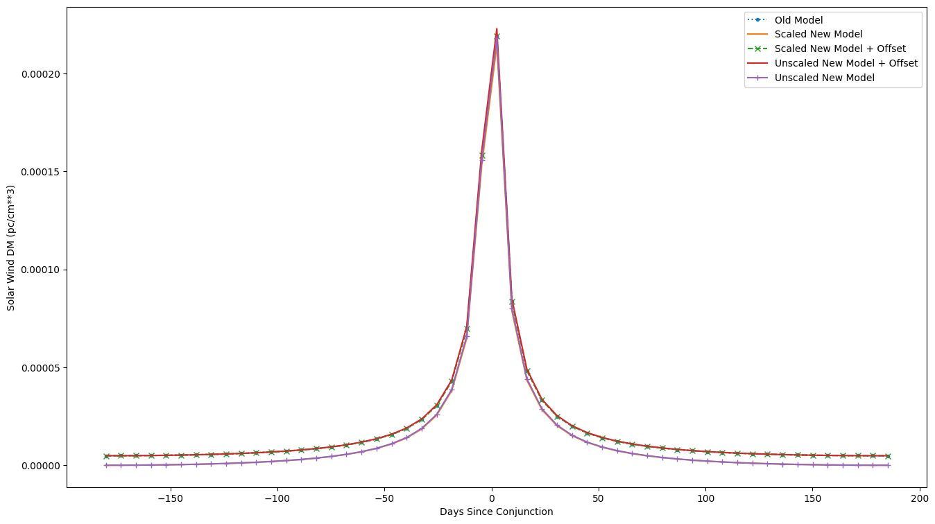
SW model limits & scalings
With the new SWX model, since it is only excess DM that starts at 0, in order to make the new model agree with the old you may need to scale some quantities
[10]:
# default model
model = get_model(StringIO("\n".join([par, "NE_SW 1"])))
# SWX model with a single segment to match the default model
model2 = get_model(
    StringIO(
        "\n".join(
            [par, "SWXDM_0001 1\nSWXP_0001 2\nSWXR1_0001 53999\nSWXR2_0001 55000"]
        )
    )
)
# because of the way SWX is scaled, scale the input
scale = model2.get_swscalings()[0]
model2.SWXDM_0001.quantity = model.get_max_dm() * scale
toas = make_fake_toas_uniform(54000, 54000 + 365.25, 53, model=model, obs="gbt")

t0, elongation = pint.utils.get_conjunction(
    model.get_psr_coords(),
    Time(54000, format="mjd"),
    precision="high",
)

x = toas.get_mjds().value - t0.mjd
fig, ax = plt.subplots(figsize=(16, 9))
ax.plot(x, model.solar_wind_dm(toas), ".:", label="Old Model")
ax.plot(x, model2.swx_dm(toas), label="Scaled New Model")
ax.plot(
    x,
    model2.swx_dm(toas) + model.get_min_dm(),
    "x--",
    label="Scaled New Model + Offset",
)
model2.SWXDM_0001.quantity = model.get_max_dm()
ax.plot(
    x,
    model2.swx_dm(toas) + model.get_min_dm(),
    label="Unscaled New Model + Offset",
)
ax.plot(
    x,
    model2.swx_dm(toas),
    "+-",
    label="Unscaled New Model",
)
ax.set_xlabel("Days Since Conjunction")
ax.set_ylabel("Solar Wind DM (pc/cm**3)")
ax.legend()
WARNING  (pint.models.model_builder     ): UNITS is not specified. Assuming TDB...
WARNING  (pint.models.model_builder     ): UNITS is not specified. Assuming TDB...
WARNING  (pint.models.absolute_phase    ): TZRMJD is not set.  Setting TZRMJD to first TOA after PEPOCH or last TOA before PEPOCH.  This may leave your residuals with an offset.
[10]:
<matplotlib.legend.Legend at 0x7ec373927a50>
Utility functions
A few functions to help move between models or separate model SWX segments
Find the next conjunction (time of SW max)
The low precision version just interpolates the Sun’s ecliptic longitude to match that of the pulsar. The high precision version uses better coordinate conversions to do this. It also returns the elongation at conjunction
[11]:
t0, elongation = pint.utils.get_conjunction(
    model.get_psr_coords(),
    Time(54000, format="mjd"),
    precision="high",
)
print(f"Next conjunction at {t0}, with elongation {elongation}")
Next conjunction at 54180.10961473882, with elongation 2.9999638108834494 deg
As expected, the elongation is just about 3 degrees (the ecliptic latitude of the pulsar)
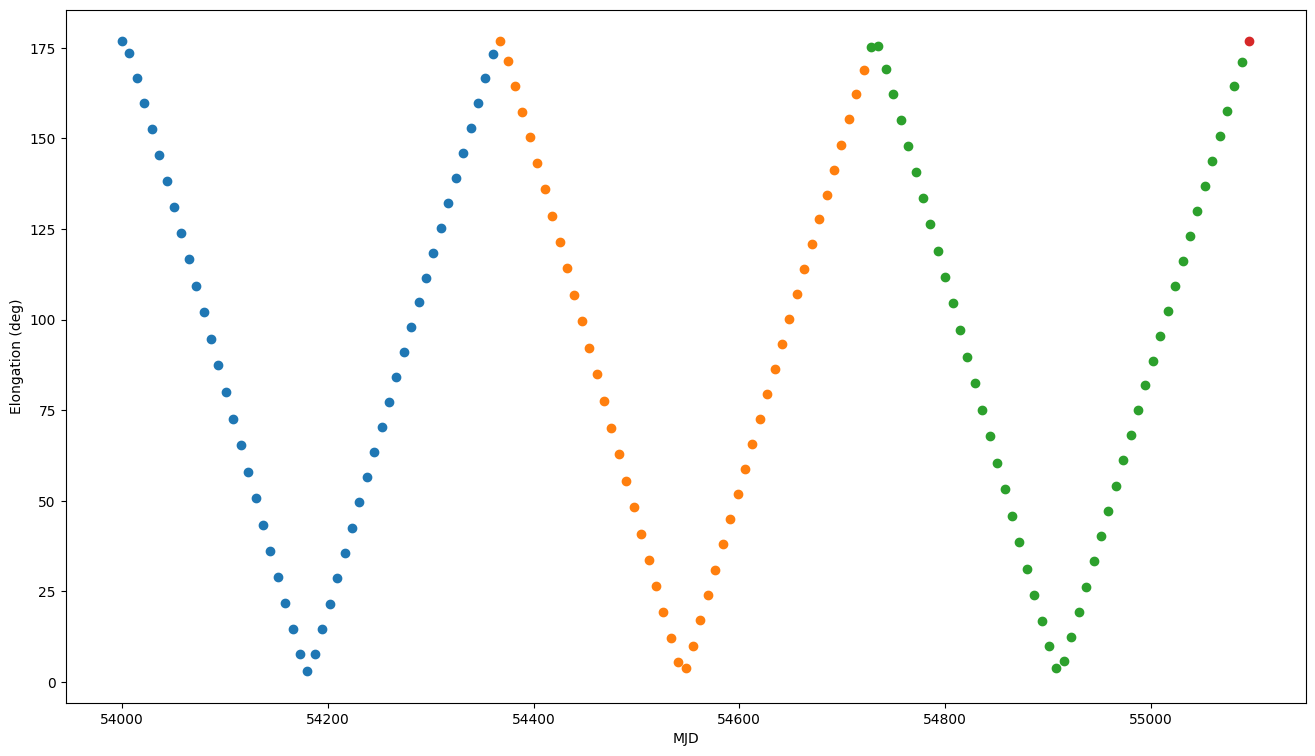
Divide the input times (TOAs) into years centered on each conjunction
This returns integer indices for each year
[12]:
toas = make_fake_toas_uniform(54000, 54000 + 365.25 * 3, 153, model=model, obs="gbt")
elongation = astropy.coordinates.get_sun(
    Time(toas.get_mjds(), format="mjd")
).separation(model.get_psr_coords())
t0 = pint.utils.get_conjunction(
    model.get_psr_coords(), model.PEPOCH.quantity, precision="high"
)[0]
indices = pint.utils.divide_times(Time(toas.get_mjds(), format="mjd"), t0)
fig, ax = plt.subplots(figsize=(16, 9))
for i in np.unique(indices):
    ax.plot(toas.get_mjds()[indices == i], elongation[indices == i].value, "o")
ax.set_xlabel("MJD")
ax.set_ylabel("Elongation (deg)")
WARNING  (pint.logging                  ): /home/docs/checkouts/readthedocs.org/user_builds/nanograv-pint/envs/1934/lib/python3.11/site-packages/astropy/coordinates/baseframe.py:1971 NonRotationTransformationWarning: transforming other coordinates from <PulsarEcliptic Frame (obliquity=84381.406 arcsec)> to <GCRS Frame (obstime=[54000.00000228 54007.20888538 54014.41776407 54021.62664773
 54028.83552214 54036.04440683 54043.25328474 54050.46217192
 54057.67104911 54064.87993063 54072.08881814 54079.29770109
 54086.5065801  54093.71545491 54100.92433672 54108.13322592
 54115.34209982 54122.55098159 54129.75987218 54136.9687514
 54144.17763439 54151.38651315 54158.5953928  54165.80428124
 54173.0131526  54180.22203899 54187.43091641 54194.6397984
 54201.84868781 54209.05756446 54216.2664444  54223.47533428
 54230.68420667 54237.89309205 54245.10197561 54252.31085532
 54259.51974094 54266.7286191  54273.93750009 54281.14638265
 54288.3552653  54295.56414655 54302.77302503 54309.98190987
 54317.19078621 54324.39967404 54331.60855829 54338.81743354
 54346.02631608 54353.2351992  54360.44407551 54367.65295827
 54374.86184734 54382.07071945 54389.27960837 54396.48848737
 54403.69737411 54410.90625154 54418.11513645 54425.32400882
 54432.53289343 54439.74178047 54446.95065958 54454.15954245
 54461.36841712 54468.57730678 54475.78618833 54482.99506194
 54490.20395172 54497.41282468 54504.62170612 54511.8305879
 54519.03947532 54526.24835146 54533.45723466 54540.66612199
 54547.87500148 54555.08388502 54562.29276169 54569.50164564
 54576.71053041 54583.91940994 54591.12828962 54598.33717642
 54605.54605622 54612.75493807 54619.96381892 54627.17269673
 54634.3815823  54641.59046292 54648.79933676 54656.00822548
 54663.21710473 54670.42598416 54677.63487278 54684.84374455
 54692.05263055 54699.26151451 54706.47039119 54713.67927773
 54720.88815473 54728.09703622 54735.30592425 54742.51480827
 54749.72368673 54756.93256821 54764.1414496  54771.35032667
 54778.5592157  54785.7680968  54792.9769736  54800.18586051
 54807.39473505 54814.60362017 54821.81250496 54829.02137839
 54836.2302631  54843.43914696 54850.64803081 54857.85690453
 54865.06579291 54872.27467537 54879.48355609 54886.69242869
 54893.90131116 54901.11020001 54908.31908151 54915.52796604
 54922.73684261 54929.94572536 54937.15460599 54944.36348829
 54951.5723663  54958.78124758 54965.99012809 54973.19901523
 54980.40789478 54987.61677732 54994.82566115 55002.03454391
 55009.24342419 55016.4523017  55023.66118661 55030.87006484
 55038.07894581 55045.28782769 55052.49670731 55059.7055918
 55066.91447637 55074.12335568 55081.33223451 55088.5411164
 55095.75000398], obsgeoloc=(0., 0., 0.) m, obsgeovel=(0., 0., 0.) m / s)>. Angular separation can depend on the direction of the transformation.
[12]:
Text(0, 0.5, 'Elongation (deg)')
Get max/min DM from standard model, or NE_SW from SWX model
[13]:
model0 = get_model(StringIO("\n".join([par, "NE_SW 30\nSWM 0"])))
# standard model with variable index
model1 = get_model(StringIO("\n".join([par, "NE_SW 30\nSWM 1\nSWP 2.5"])))
# SWX model with 1 segment
model2 = get_model(
    StringIO(
        "\n".join(
            [par, "SWXDM_0001 1\nSWXP_0001 2\nSWXR1_0001 53999\nSWXR2_0001 55000"]
        )
    )
)
# one value of the scale is returned for each SWX segment
scale = model2.get_swscalings()[0]
print(f"SW scaling: {scale}")
model2.SWXDM_0001.quantity = model0.get_max_dm() * scale
WARNING  (pint.models.model_builder     ): UNITS is not specified. Assuming TDB...
WARNING  (pint.models.model_builder     ): UNITS is not specified. Assuming TDB...
WARNING  (pint.models.model_builder     ): UNITS is not specified. Assuming TDB...
SW scaling: 0.9830510553813481
[14]:
# Max is at conjunction, Min at opposition
print(
    f"SWM=0: NE_SW = {model0.NE_SW.quantity:.2f} Max DM = {model0.get_max_dm():.4f}, Min DM = {model0.get_min_dm():.4f}"
)
# Max and Min depend on NE_SW and SWP (covariance)
print(
    f"SWM=1 and SWP={model1.SWP.value}:  NE_SW = {model1.NE_SW.quantity:.2f} Max DM = {model1.get_max_dm():.4f}, Min DM = {model1.get_min_dm():.4f}"
)
# For SWX, the max/min values reported do not assume that it goes to 0 at opposition (for compatibility)
print(
    f"SWX and SWP={model2.SWXP_0001.value}: NE_SW = {model2.get_ne_sws()[0]:.2f} Max DM = {model2.get_max_dms()[0]:.4f}, Min DM = {model2.get_min_dms()[0]:.4f}"
)
print(
    f"SWX and SWP={model2.SWXP_0001.value}: Scaled NE_SW = {model2.get_ne_sws()[0]/scale:.2f} Scaled Max DM = {model2.get_max_dms()[0]/scale:.4f}, Scaled Min DM = {model2.get_min_dms()[0]/scale:.4f}"
)
SWM=0: NE_SW = 30.00 1 / cm3 Max DM = 0.0086 pc / cm3, Min DM = 0.0001 pc / cm3
SWM=1 and SWP=2.5:  NE_SW = 30.00 1 / cm3 Max DM = 0.0290 pc / cm3, Min DM = 0.0001 pc / cm3
SWX and SWP=2.0: NE_SW = 29.49 1 / cm3 Max DM = 0.0084 pc / cm3, Min DM = 0.0001 pc / cm3
SWX and SWP=2.0: Scaled NE_SW = 30.00 1 / cm3 Scaled Max DM = 0.0086 pc / cm3, Scaled Min DM = 0.0001 pc / cm3
The scaled values above agree between the SWM=0 and SWX models.
[ ]: