This Jupyter notebook can be downloaded from rednoise-fit-example.ipynb, or viewed as a python script at rednoise-fit-example.py.
Red noise, DM noise, and chromatic noise fitting examples
This notebook provides an example on how to fit for red noise and DM noise using PINT using simulated datasets.
We will use the PLRedNoise and PLDMNoise models to generate noise realizations (these models provide Fourier Gaussian process descriptions of achromatic red noise and DM noise respectively).
We will fit the generated datasets using the WaveX and DMWaveX models, which provide deterministic Fourier representations of achromatic red noise and DM noise respectively.
Finally, we will convert the WaveX/DMWaveX amplitudes into spectral parameters and compare them with the injected values.
[1]:
from pint import DMconst
from pint.models import get_model
from pint.simulation import make_fake_toas_uniform
from pint.logging import setup as setup_log
from pint.fitter import WLSFitter
from pint.utils import (
    cmwavex_setup,
    dmwavex_setup,
    find_optimal_nharms,
    plchromnoise_from_cmwavex,
    wavex_setup,
    plrednoise_from_wavex,
    pldmnoise_from_dmwavex,
)

from io import StringIO
import numpy as np
import astropy.units as u
from matplotlib import pyplot as plt
from copy import deepcopy

setup_log(level="WARNING")
[1]:
1
Red noise fitting
Simulation
The first step is to generate a simulated dataset for demonstration. Note that we are adding PHOFF as a free parameter. This is required for the fit to work properly.
[2]:
par_sim = """
    PSR           SIM3
    RAJ           05:00:00     1
    DECJ          15:00:00     1
    PEPOCH        55000
    F0            100          1
    F1            -1e-15       1
    PHOFF         0            1
    DM            15           1
    TNREDAMP      -13
    TNREDGAM      3.5
    TNREDC        30
    TZRMJD        55000
    TZRFRQ        1400
    TZRSITE       gbt
    UNITS         TDB
    EPHEM         DE440
    CLOCK         TT(BIPM2019)
"""

m = get_model(StringIO(par_sim))
[3]:
# Now generate the simulated TOAs.
ntoas = 2000
toaerrs = np.random.uniform(0.5, 2.0, ntoas) * u.us
freqs = np.linspace(500, 1500, 8) * u.MHz

t = make_fake_toas_uniform(
    startMJD=53001,
    endMJD=57001,
    ntoas=ntoas,
    model=m,
    freq=freqs,
    obs="gbt",
    error=toaerrs,
    add_noise=True,
    add_correlated_noise=True,
    name="fake",
    include_bipm=True,
    multi_freqs_in_epoch=True,
)
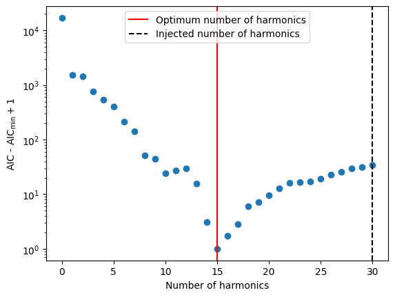
Optimal number of harmonics
The optimal number of harmonics can be estimated by minimizing the Akaike Information Criterion (AIC). This is implemented in the pint.utils.find_optimal_nharms function.
[4]:
m1 = deepcopy(m)
m1.remove_component("PLRedNoise")

nharm_opt, d_aics = find_optimal_nharms(m1, t, "WaveX", 30)

print("Optimum no of harmonics = ", nharm_opt)
Optimum no of harmonics = 17
[5]:
print(np.argmin(d_aics))
17
[6]:
# The Y axis is plotted in log scale only for better visibility.
plt.scatter(list(range(len(d_aics))), d_aics + 1)
plt.axvline(nharm_opt, color="red", label="Optimum number of harmonics")
plt.axvline(
    int(m.TNREDC.value), color="black", ls="--", label="Injected number of harmonics"
)
plt.xlabel("Number of harmonics")
plt.ylabel("AIC - AIC$_\\min{} + 1$")
plt.legend()
plt.yscale("log")
# plt.savefig("sim3-aic.pdf")
[7]:
# Now create a new model with the optimum number of harmonics
m2 = deepcopy(m1)
Tspan = t.get_mjds().max() - t.get_mjds().min()
wavex_setup(m2, T_span=Tspan, n_freqs=nharm_opt, freeze_params=False)

ftr = WLSFitter(t, m2)
ftr.fit_toas(maxiter=10)
m2 = ftr.model

print(m2)
# Created: 2026-02-25T11:52:28.808898
# PINT_version: 1.1.4+67.g3113e81
# User: docs
# Host: build-31553150-project-85767-nanograv-pint
# OS: Linux-6.8.0-1029-aws-x86_64-with-glibc2.35
# Python: 3.11.12 (main, May  6 2025, 10:45:53) [GCC 11.4.0]
# Format: pint
# read_time: 2026-02-25T11:51:53.076497
# allow_tcb: False
# convert_tcb: False
# allow_T2: False
PSR                                  SIM3
EPHEM                               DE440
CLOCK                        TT(BIPM2019)
UNITS                                 TDB
START              53000.9999999567360532
FINISH             56985.0000000464880093
DILATEFREQ                              N
DMDATA                                  N
NTOA                                 2000
CHI2                   1870.6303301989212
CHI2R                  0.9548904186824508
TRES               0.95634496917142042255
RAJ                      5:00:00.00010288 1 0.00011008674976652021
DECJ                    14:59:59.98380586 1 0.01171456276922400175
PMRA                                  0.0
PMDEC                                 0.0
PX                                    0.0
F0                   100.0000000000001244 1 5.0470770597470997634e-13
F1              -9.9980797331508296875e-16 1 1.7827097864176728477e-19
PEPOCH             55000.0000000000000000
PLANET_SHAPIRO                          N
DM                   15.00000485472122553 1 4.7077963841564644172e-06
WXEPOCH            55000.0000000000000000
WXFREQ_0001        0.00025100401605860257
WXSIN_0001        -3.6129688669821524e-06 1 5.665545108191531e-07
WXCOS_0001        -1.1547010150239786e-05 1 1.0770601466718245e-05
WXFREQ_0002         0.0005020080321172051
WXSIN_0002         1.3436315266693063e-07 1 2.8572390838104384e-07
WXCOS_0002          2.429290430140687e-06 1 2.7385452438294782e-06
WXFREQ_0003         0.0007530120481758077
WXSIN_0003         1.4971792948727635e-07 1 1.9904529541902517e-07
WXCOS_0003        -3.0320308301881253e-06 1 1.2553296576318186e-06
WXFREQ_0004         0.0010040160642344103
WXSIN_0004         1.2427588093298467e-06 1 1.5930892672524627e-07
WXCOS_0004         1.4607516075513943e-06 1 7.398398864032494e-07
WXFREQ_0005         0.0012550200802930128
WXSIN_0005          2.472544394585756e-07 1 1.3783060174845877e-07
WXCOS_0005         -9.011828403210133e-07 1 5.061492922425036e-07
WXFREQ_0006         0.0015060240963516154
WXSIN_0006         -1.692796172870195e-07 1 1.291775893888326e-07
WXCOS_0006          5.300668545752909e-07 1 3.869692342671927e-07
WXFREQ_0007          0.001757028112410218
WXSIN_0007          8.321008082297241e-08 1 1.2871365883955333e-07
WXCOS_0007          -3.91229906634015e-07 1 3.2471570790020947e-07
WXFREQ_0008         0.0020080321284688205
WXSIN_0008           1.74981488947027e-08 1 1.3958293731047164e-07
WXCOS_0008          4.113016660909747e-07 1 3.016440296779882e-07
WXFREQ_0009         0.0022590361445274233
WXSIN_0009          4.918682520486656e-08 1 1.7188964007497925e-07
WXCOS_0009        -4.3868405234703357e-07 1 3.283904449238054e-07
WXFREQ_0010         0.0025100401605860257
WXSIN_0010        -5.0107162860086114e-08 1 3.001053262776854e-07
WXCOS_0010          8.380637179409308e-07 1 5.005232340874728e-07
WXFREQ_0011         0.0027610441766446284
WXSIN_0011        -4.6923517286555644e-07 1 2.4671447266907553e-06
WXCOS_0011          5.034065560018563e-06 1 3.614022061068006e-06
WXFREQ_0012          0.003012048192703231
WXSIN_0012         -9.025697701933414e-08 1 1.7984756745321769e-07
WXCOS_0012         -3.162478869127971e-07 1 2.3156795254484863e-07
WXFREQ_0013         0.0032630522087618336
WXSIN_0013         2.2599785840914836e-08 1 8.64100897536497e-08
WXCOS_0013         1.7246171831670624e-07 1 9.715026023860558e-08
WXFREQ_0014          0.003514056224820436
WXSIN_0014         1.6680070076765218e-07 1 5.597352607083803e-08
WXCOS_0014          6.841998257664027e-08 1 5.6521881045986636e-08
WXFREQ_0015         0.0037650602408790387
WXSIN_0015         -8.858192577070503e-08 1 4.331545793275323e-08
WXCOS_0015         -5.201812747479837e-08 1 4.303799671319005e-08
WXFREQ_0016          0.004016064256937641
WXSIN_0016         -9.687350751444101e-08 1 3.800843137467801e-08
WXCOS_0016          7.619244202041802e-08 1 3.705076119779324e-08
WXFREQ_0017          0.004267068272996243
WXSIN_0017        -5.7207341453234813e-08 1 3.579791263773082e-08
WXCOS_0017         -7.919000476876842e-08 1 3.451615988979281e-08
TZRMJD             55000.0000000000000000
TZRSITE                               gbt
TZRFRQ                             1400.0
PHOFF             -0.00014660909417449133 1 0.0008909062596210944
Estimating the spectral parameters from the WaveX fit.
[8]:
# Get the Fourier amplitudes and powers and their uncertainties.
idxs = np.array(m2.components["WaveX"].get_indices())
a = np.array([m2[f"WXSIN_{idx:04d}"].quantity.to_value("s") for idx in idxs])
da = np.array([m2[f"WXSIN_{idx:04d}"].uncertainty.to_value("s") for idx in idxs])
b = np.array([m2[f"WXCOS_{idx:04d}"].quantity.to_value("s") for idx in idxs])
db = np.array([m2[f"WXCOS_{idx:04d}"].uncertainty.to_value("s") for idx in idxs])
print(len(idxs))

P = (a**2 + b**2) / 2
dP = ((a * da) ** 2 + (b * db) ** 2) ** 0.5

f0 = (1 / Tspan).to_value(u.Hz)
fyr = (1 / u.year).to_value(u.Hz)
17
[9]:
# We can create a `PLRedNoise` model from the `WaveX` model.
# This will estimate the spectral parameters from the `WaveX`
# amplitudes.
m3 = plrednoise_from_wavex(m2)
print(m3)
# Created: 2026-02-25T11:52:28.840225
# PINT_version: 1.1.4+67.g3113e81
# User: docs
# Host: build-31553150-project-85767-nanograv-pint
# OS: Linux-6.8.0-1029-aws-x86_64-with-glibc2.35
# Python: 3.11.12 (main, May  6 2025, 10:45:53) [GCC 11.4.0]
# Format: pint
# read_time: 2026-02-25T11:51:53.076497
# allow_tcb: False
# convert_tcb: False
# allow_T2: False
PSR                                  SIM3
EPHEM                               DE440
CLOCK                        TT(BIPM2019)
UNITS                                 TDB
START              53000.9999999567360532
FINISH             56985.0000000464880093
DILATEFREQ                              N
DMDATA                                  N
NTOA                                 2000
CHI2                   1870.6303301989212
CHI2R                  0.9548904186824508
TRES               0.95634496917142042255
RAJ                      5:00:00.00010288 1 0.00011008674976652021
DECJ                    14:59:59.98380586 1 0.01171456276922400175
PMRA                                  0.0
PMDEC                                 0.0
PX                                    0.0
F0                   100.0000000000001244 1 5.0470770597470997634e-13
F1              -9.9980797331508296875e-16 1 1.7827097864176728477e-19
PEPOCH             55000.0000000000000000
PLANET_SHAPIRO                          N
DM                   15.00000485472122553 1 4.7077963841564644172e-06
TNREDAMP              -12.850165327732267 0 0.10193350233150412
TNREDGAM               3.0134763717172453 0 0.5389509980755075
TNREDC                                 17
TZRMJD             55000.0000000000000000
TZRSITE                               gbt
TZRFRQ                             1400.0
PHOFF             -0.00014660909417449133 1 0.0008909062596210944
[10]:
# Now let us plot the estimated spectrum with the injected
# spectrum.
plt.subplot(211)
plt.errorbar(
    idxs * f0,
    b * 1e6,
    db * 1e6,
    ls="",
    marker="o",
    label="$\\hat{a}_j$ (WXCOS)",
    color="red",
)
plt.errorbar(
    idxs * f0,
    a * 1e6,
    da * 1e6,
    ls="",
    marker="o",
    label="$\\hat{b}_j$ (WXSIN)",
    color="blue",
)
plt.axvline(fyr, color="black", ls="dotted")
plt.axhline(0, color="grey", ls="--")
plt.ylabel("Fourier coeffs ($\mu$s)")
plt.xscale("log")
plt.legend(fontsize=8)

plt.subplot(212)
plt.errorbar(
    idxs * f0, P, dP, ls="", marker="o", label="Spectral power (PINT)", color="k"
)
P_inj = m.components["PLRedNoise"].get_noise_weights(t)[::2][:nharm_opt]
plt.plot(idxs * f0, P_inj, label="Injected Spectrum", color="r")
P_est = m3.components["PLRedNoise"].get_noise_weights(t)[::2][:nharm_opt]
print(len(idxs), len(P_est))
plt.plot(idxs * f0, P_est, label="Estimated Spectrum", color="b")
plt.xscale("log")
plt.yscale("log")
plt.ylabel("Spectral power (s$^2$)")
plt.xlabel("Frequency (Hz)")
plt.axvline(fyr, color="black", ls="dotted", label="1 yr$^{-1}$")
plt.legend()
17 17
[10]:
<matplotlib.legend.Legend at 0x710ec3da40d0>
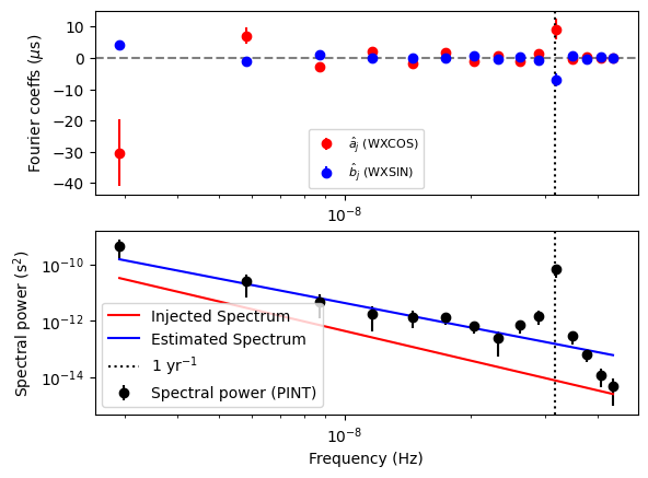
Note the outlier in the 1 year^-1 bin. This is caused by the covariance with RA and DEC, which introduce a delay with the same frequency.
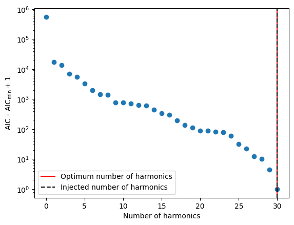
DM noise fitting
Let us now do a similar kind of analysis for DM noise.
[11]:
par_sim = """
    PSR           SIM4
    RAJ           05:00:00     1
    DECJ          15:00:00     1
    PEPOCH        55000
    F0            100          1
    F1            -1e-15       1
    PHOFF         0            1
    DM            15           1
    TNDMAMP       -13
    TNDMGAM       3.5
    TNDMC         30
    TZRMJD        55000
    TZRFRQ        1400
    TZRSITE       gbt
    UNITS         TDB
    EPHEM         DE440
    CLOCK         TT(BIPM2019)
"""

m = get_model(StringIO(par_sim))
[12]:
# Generate the simulated TOAs.
ntoas = 2000
toaerrs = np.random.uniform(0.5, 2.0, ntoas) * u.us
freqs = np.linspace(500, 1500, 8) * u.MHz

t = make_fake_toas_uniform(
    startMJD=53001,
    endMJD=57001,
    ntoas=ntoas,
    model=m,
    freq=freqs,
    obs="gbt",
    error=toaerrs,
    add_noise=True,
    add_correlated_noise=True,
    name="fake",
    include_bipm=True,
    multi_freqs_in_epoch=True,
)
[13]:
# Find the optimum number of harmonics by minimizing AIC.
m1 = deepcopy(m)
m1.remove_component("PLDMNoise")

m2 = deepcopy(m1)

nharm_opt, d_aics = find_optimal_nharms(m2, t, "DMWaveX", 30)
print("Optimum no of harmonics = ", nharm_opt)
Optimum no of harmonics = 30
[14]:
# The Y axis is plotted in log scale only for better visibility.
plt.scatter(list(range(len(d_aics))), d_aics + 1)
plt.axvline(nharm_opt, color="red", label="Optimum number of harmonics")
plt.axvline(
    int(m.TNDMC.value), color="black", ls="--", label="Injected number of harmonics"
)
plt.xlabel("Number of harmonics")
plt.ylabel("AIC - AIC$_\\min{} + 1$")
plt.legend()
plt.yscale("log")
# plt.savefig("sim3-aic.pdf")
[15]:
# Now create a new model with the optimum number of
# harmonics
m2 = deepcopy(m1)

Tspan = t.get_mjds().max() - t.get_mjds().min()
dmwavex_setup(m2, T_span=Tspan, n_freqs=nharm_opt, freeze_params=False)

ftr = WLSFitter(t, m2)
ftr.fit_toas(maxiter=10)
m2 = ftr.model

print(m2)
# Created: 2026-02-25T11:53:11.068283
# PINT_version: 1.1.4+67.g3113e81
# User: docs
# Host: build-31553150-project-85767-nanograv-pint
# OS: Linux-6.8.0-1029-aws-x86_64-with-glibc2.35
# Python: 3.11.12 (main, May  6 2025, 10:45:53) [GCC 11.4.0]
# Format: pint
# read_time: 2026-02-25T11:52:29.229804
# allow_tcb: False
# convert_tcb: False
# allow_T2: False
PSR                                  SIM4
EPHEM                               DE440
CLOCK                        TT(BIPM2019)
UNITS                                 TDB
START              53000.9999999566624884
FINISH             56985.0000000460339120
DILATEFREQ                              N
DMDATA                                  N
NTOA                                 2000
CHI2                    1923.453436287121
CHI2R                  0.9950612707124267
TRES               0.99344541007098360224
RAJ                      4:59:59.99999754 1 0.00000190874270482314
DECJ                    14:59:59.99996787 1 0.00016496453926019566
PMRA                                  0.0
PMDEC                                 0.0
PX                                    0.0
F0                  100.00000000000000648 1 3.6266194848918145154e-14
F1              -1.0000004034504575966e-15 1 8.422704923186267577e-22
PEPOCH             55000.0000000000000000
PLANET_SHAPIRO                          N
DM                  15.000000216915388534 1 5.0749015207111111675e-06
DMWXEPOCH          55000.0000000000000000
DMWXFREQ_0001       0.0002510040160586264
DMWXSIN_0001        0.0029148834374415115 1 6.052932059413716e-06
DMWXCOS_0001         0.004728696548000313 1 7.044147848987271e-06
DMWXFREQ_0002       0.0005020080321172528
DMWXSIN_0002       3.6472223996336825e-05 1 4.9206796549811355e-06
DMWXCOS_0002        0.0009053056367664808 1 4.5532577331280654e-06
DMWXFREQ_0003       0.0007530120481758793
DMWXSIN_0003       -0.0008124412055853551 1 4.6326856054154035e-06
DMWXCOS_0003       -0.0011704053480140887 1 4.423431586087979e-06
DMWXFREQ_0004       0.0010040160642345057
DMWXSIN_0004      -0.00014420586358654944 1 4.600619026219083e-06
DMWXCOS_0004       0.00037735184542007764 1 4.345772634947938e-06
DMWXFREQ_0005        0.001255020080293132
DMWXSIN_0005       0.00032447690202913875 1 4.508719827276058e-06
DMWXCOS_0005       -6.826532989249648e-05 1 4.348086253420156e-06
DMWXFREQ_0006       0.0015060240963517585
DMWXSIN_0006       1.6353123573178224e-05 1 4.434479068820563e-06
DMWXCOS_0006      -1.2655387453854644e-05 1 4.376527723603912e-06
DMWXFREQ_0007        0.001757028112410385
DMWXSIN_0007       -1.911289972521748e-05 1 4.457509895712002e-06
DMWXCOS_0007       -8.119859808514635e-05 1 4.352764840279056e-06
DMWXFREQ_0008       0.0020080321284690113
DMWXSIN_0008        8.975004658194116e-05 1 4.368523005076918e-06
DMWXCOS_0008         7.79653651621098e-05 1 4.426022327391967e-06
DMWXFREQ_0009       0.0022590361445276375
DMWXSIN_0009       -2.917661497094915e-05 1 4.4095045855440026e-06
DMWXCOS_0009       4.6239283091658414e-05 1 4.382529010932787e-06
DMWXFREQ_0010        0.002510040160586264
DMWXSIN_0010         0.000108498825604401 1 4.441558290588034e-06
DMWXCOS_0010       1.8847157869107666e-05 1 4.3933588711604455e-06
DMWXFREQ_0011       0.0027610441766448904
DMWXSIN_0011      -2.2404193238783096e-05 1 7.0216944008445495e-06
DMWXCOS_0011        4.053119456470124e-05 1 7.129684613285063e-06
DMWXFREQ_0012        0.003012048192703517
DMWXSIN_0012       1.4282455471381412e-05 1 4.388343706152251e-06
DMWXCOS_0012       -5.861060871911731e-05 1 4.40855141776485e-06
DMWXFREQ_0013        0.003263052208762143
DMWXSIN_0013       1.6013758567482416e-05 1 4.416712255921489e-06
DMWXCOS_0013      -4.8886174306877924e-05 1 4.331731688741734e-06
DMWXFREQ_0014         0.00351405622482077
DMWXSIN_0014        2.765028933688814e-05 1 4.440338872730756e-06
DMWXCOS_0014       -4.672407140179151e-05 1 4.325485748809395e-06
DMWXFREQ_0015        0.003765060240879396
DMWXSIN_0015      -2.9891856324401605e-05 1 4.30929680785618e-06
DMWXCOS_0015       6.0921657624368945e-06 1 4.427407543048835e-06
DMWXFREQ_0016        0.004016064256938023
DMWXSIN_0016        7.842882846246635e-06 1 4.41369433515517e-06
DMWXCOS_0016       -1.691689219675711e-05 1 4.331617089229114e-06
DMWXFREQ_0017        0.004267068272996649
DMWXSIN_0017         2.26428809027135e-05 1 4.370767980164771e-06
DMWXCOS_0017       -7.705230774694198e-06 1 4.374234104174039e-06
DMWXFREQ_0018        0.004518072289055275
DMWXSIN_0018       -2.064015862523369e-05 1 4.354797374993665e-06
DMWXCOS_0018      -1.1048811242929405e-05 1 4.38313716572353e-06
DMWXFREQ_0019        0.004769076305113902
DMWXSIN_0019       1.7769757119682563e-05 1 4.423526837236385e-06
DMWXCOS_0019       -2.956352278364193e-07 1 4.32478417925469e-06
DMWXFREQ_0020        0.005020080321172528
DMWXSIN_0020      -1.7674442452724775e-05 1 4.408690628268063e-06
DMWXCOS_0020       3.3231393995235926e-05 1 4.3430680784770934e-06
DMWXFREQ_0021        0.005271084337231155
DMWXSIN_0021       1.3631831449951883e-06 1 4.424239653635454e-06
DMWXCOS_0021       3.9251982039166324e-06 1 4.326178066958088e-06
DMWXFREQ_0022        0.005522088353289781
DMWXSIN_0022       1.5201741171858495e-05 1 4.440740018130212e-06
DMWXCOS_0022       1.2282030819849575e-05 1 4.323211252270374e-06
DMWXFREQ_0023        0.005773092369348407
DMWXSIN_0023       2.4164715590510993e-06 1 4.386530747613683e-06
DMWXCOS_0023        6.567413780236557e-06 1 4.372669646097008e-06
DMWXFREQ_0024        0.006024096385407034
DMWXSIN_0024       -6.291791923062014e-07 1 4.425414015712667e-06
DMWXCOS_0024        -7.79590011016509e-06 1 4.343632894619493e-06
DMWXFREQ_0025        0.006275100401465661
DMWXSIN_0025         6.17194209993774e-06 1 4.43349076340757e-06
DMWXCOS_0025      -1.2019935491255281e-05 1 4.334318264081869e-06
DMWXFREQ_0026        0.006526104417524286
DMWXSIN_0026        1.503836168842577e-05 1 4.235031284070854e-06
DMWXCOS_0026       -7.471012958122823e-07 1 4.521056573509654e-06
DMWXFREQ_0027        0.006777108433582913
DMWXSIN_0027       -1.652609168334414e-05 1 4.431465864088462e-06
DMWXCOS_0027       1.1515682476561766e-05 1 4.318372384248246e-06
DMWXFREQ_0028         0.00702811244964154
DMWXSIN_0028         -4.5615564787784e-06 1 4.317181368632052e-06
DMWXCOS_0028       -7.068049332227934e-06 1 4.427253019279415e-06
DMWXFREQ_0029        0.007279116465700166
DMWXSIN_0029      -2.2969168551586415e-06 1 4.346975069147191e-06
DMWXCOS_0029       -8.130195814182882e-06 1 4.389517626106801e-06
DMWXFREQ_0030        0.007530120481758792
DMWXSIN_0030        9.256887985116869e-06 1 4.371561792335194e-06
DMWXCOS_0030      -5.5893524256794076e-06 1 4.364377606550752e-06
TZRMJD             55000.0000000000000000
TZRSITE                               gbt
TZRFRQ                             1400.0
PHOFF               0.0009940063647874097 1 5.6823019444730265e-06
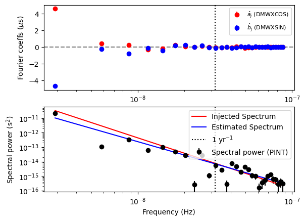
Estimating the spectral parameters from the DMWaveX fit.
[16]:
# Get the Fourier amplitudes and powers and their uncertainties.
# Note that the `DMWaveX` amplitudes have the units of DM.
# We multiply them by a constant factor to convert them to dimensions
# of time so that they are consistent with `PLDMNoise`.
scale = DMconst / (1400 * u.MHz) ** 2

idxs = np.array(m2.components["DMWaveX"].get_indices())
a = np.array(
    [(scale * m2[f"DMWXSIN_{idx:04d}"].quantity).to_value("s") for idx in idxs]
)
da = np.array(
    [(scale * m2[f"DMWXSIN_{idx:04d}"].uncertainty).to_value("s") for idx in idxs]
)
b = np.array(
    [(scale * m2[f"DMWXCOS_{idx:04d}"].quantity).to_value("s") for idx in idxs]
)
db = np.array(
    [(scale * m2[f"DMWXCOS_{idx:04d}"].uncertainty).to_value("s") for idx in idxs]
)
print(len(idxs))

P = (a**2 + b**2) / 2
dP = ((a * da) ** 2 + (b * db) ** 2) ** 0.5

f0 = (1 / Tspan).to_value(u.Hz)
fyr = (1 / u.year).to_value(u.Hz)
30
[17]:
# We can create a `PLDMNoise` model from the `DMWaveX` model.
# This will estimate the spectral parameters from the `DMWaveX`
# amplitudes.
m3 = pldmnoise_from_dmwavex(m2)
print(m3)
# Created: 2026-02-25T11:53:11.108011
# PINT_version: 1.1.4+67.g3113e81
# User: docs
# Host: build-31553150-project-85767-nanograv-pint
# OS: Linux-6.8.0-1029-aws-x86_64-with-glibc2.35
# Python: 3.11.12 (main, May  6 2025, 10:45:53) [GCC 11.4.0]
# Format: pint
# read_time: 2026-02-25T11:52:29.229804
# allow_tcb: False
# convert_tcb: False
# allow_T2: False
PSR                                  SIM4
EPHEM                               DE440
CLOCK                        TT(BIPM2019)
UNITS                                 TDB
START              53000.9999999566624884
FINISH             56985.0000000460339120
DILATEFREQ                              N
DMDATA                                  N
NTOA                                 2000
CHI2                    1923.453436287121
CHI2R                  0.9950612707124267
TRES               0.99344541007098360224
RAJ                      4:59:59.99999754 1 0.00000190874270482314
DECJ                    14:59:59.99996787 1 0.00016496453926019566
PMRA                                  0.0
PMDEC                                 0.0
PX                                    0.0
F0                  100.00000000000000648 1 3.6266194848918145154e-14
F1              -1.0000004034504575966e-15 1 8.422704923186267577e-22
PEPOCH             55000.0000000000000000
PLANET_SHAPIRO                          N
DM                  15.000000216915388534 1 5.0749015207111111675e-06
TNDMAMP               -12.959710947511473 0 0.04296666716792681
TNDMGAM                 3.891533410574481 0 0.23942316078613335
TNDMC                                  30
TZRMJD             55000.0000000000000000
TZRSITE                               gbt
TZRFRQ                             1400.0
PHOFF               0.0009940063647874097 1 5.6823019444730265e-06
[18]:
# Now let us plot the estimated spectrum with the injected
# spectrum.
plt.subplot(211)
plt.errorbar(
    idxs * f0,
    b * 1e6,
    db * 1e6,
    ls="",
    marker="o",
    label="$\\hat{a}_j$ (DMWXCOS)",
    color="red",
)
plt.errorbar(
    idxs * f0,
    a * 1e6,
    da * 1e6,
    ls="",
    marker="o",
    label="$\\hat{b}_j$ (DMWXSIN)",
    color="blue",
)
plt.axvline(fyr, color="black", ls="dotted")
plt.axhline(0, color="grey", ls="--")
plt.ylabel("Fourier coeffs ($\mu$s)")
plt.xscale("log")
plt.legend(fontsize=8)

plt.subplot(212)
plt.errorbar(
    idxs * f0, P, dP, ls="", marker="o", label="Spectral power (PINT)", color="k"
)
P_inj = m.components["PLDMNoise"].get_noise_weights(t)[::2][:nharm_opt]
plt.plot(idxs * f0, P_inj, label="Injected Spectrum", color="r")
P_est = m3.components["PLDMNoise"].get_noise_weights(t)[::2][:nharm_opt]
print(len(idxs), len(P_est))
plt.plot(idxs * f0, P_est, label="Estimated Spectrum", color="b")
plt.xscale("log")
plt.yscale("log")
plt.ylabel("Spectral power (s$^2$)")
plt.xlabel("Frequency (Hz)")
plt.axvline(fyr, color="black", ls="dotted", label="1 yr$^{-1}$")
plt.legend()
30 30
[18]:
<matplotlib.legend.Legend at 0x710ec107bbd0>
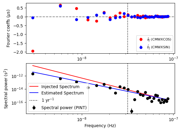
Chromatic noise fitting
Let us now do a similar kind of analysis for chromatic noise.
[19]:
par_sim = """
    PSR           SIM5
    RAJ           05:00:00     1
    DECJ          15:00:00     1
    PEPOCH        55000
    F0            100          1
    F1            -1e-15       1
    PHOFF         0            1
    DM            15
    CM            1.2          1
    TNCHROMIDX    3.5
    TNCHROMAMP    -13
    TNCHROMGAM    3.5
    TNCHROMC      30
    TZRMJD        55000
    TZRFRQ        1400
    TZRSITE       gbt
    UNITS         TDB
    EPHEM         DE440
    CLOCK         TT(BIPM2019)
"""

m = get_model(StringIO(par_sim))
[20]:
# Generate the simulated TOAs.
ntoas = 2000
toaerrs = np.random.uniform(0.5, 2.0, ntoas) * u.us
freqs = np.linspace(500, 1500, 8) * u.MHz

t = make_fake_toas_uniform(
    startMJD=53001,
    endMJD=57001,
    ntoas=ntoas,
    model=m,
    freq=freqs,
    obs="gbt",
    error=toaerrs,
    add_noise=True,
    add_correlated_noise=True,
    name="fake",
    include_bipm=True,
    multi_freqs_in_epoch=True,
)
[21]:
# Find the optimum number of harmonics by minimizing AIC.
m1 = deepcopy(m)
m1.remove_component("PLChromNoise")

m2 = deepcopy(m1)

nharm_opt = m.TNCHROMC.value
[22]:
# Now create a new model with the optimum number of
# harmonics
m2 = deepcopy(m1)

Tspan = t.get_mjds().max() - t.get_mjds().min()
cmwavex_setup(m2, T_span=Tspan, n_freqs=nharm_opt, freeze_params=False)

ftr = WLSFitter(t, m2)
ftr.fit_toas(maxiter=10)
m2 = ftr.model

print(m2)
# Created: 2026-02-25T11:53:18.355479
# PINT_version: 1.1.4+67.g3113e81
# User: docs
# Host: build-31553150-project-85767-nanograv-pint
# OS: Linux-6.8.0-1029-aws-x86_64-with-glibc2.35
# Python: 3.11.12 (main, May  6 2025, 10:45:53) [GCC 11.4.0]
# Format: pint
# read_time: 2026-02-25T11:53:11.426302
# allow_tcb: False
# convert_tcb: False
# allow_T2: False
PSR                                  SIM5
EPHEM                               DE440
CLOCK                        TT(BIPM2019)
UNITS                                 TDB
START              53000.9999999567202084
FINISH             56985.0000000475109491
DILATEFREQ                              N
DMDATA                                  N
NTOA                                 2000
CHI2                   1887.8626953637342
CHI2R                   0.976649092273013
TRES               0.95666063343806419917
RAJ                      4:59:59.99999927 1 0.00000141835301876501
DECJ                    15:00:00.00001482 1 0.00012039207992145633
PMRA                                  0.0
PMDEC                                 0.0
PX                                    0.0
F0                  100.00000000000001954 1 2.7670653170953090219e-14
F1              -1.0000007324788201994e-15 1 6.225448125407257128e-22
PEPOCH             55000.0000000000000000
PLANET_SHAPIRO                          N
DM                                   15.0
CM                  1.2152009140414240223 1 0.05008292176268339807
TNCHROMIDX                            3.5
CMWXEPOCH          55000.0000000000000000
CMWXFREQ_0001        0.000251004016058537
CMWXSIN_0001          -216.69480091679011 1 0.06600100455373246
CMWXCOS_0001          -212.89164879514018 1 0.06875777981580293
CMWXFREQ_0002        0.000502008032117074
CMWXSIN_0002           -69.49603721210072 1 0.06073050797606602
CMWXCOS_0002           -86.50743342054614 1 0.05554938026400449
CMWXFREQ_0003        0.000753012048175611
CMWXSIN_0003           -17.75234857281413 1 0.05763237675561338
CMWXCOS_0003           38.816937922011924 1 0.0567934357885569
CMWXFREQ_0004        0.001004016064234148
CMWXSIN_0004          -1.3323453718675435 1 0.05782316329684783
CMWXCOS_0004           -23.53089856229034 1 0.05605344406541237
CMWXFREQ_0005       0.0012550200802926852
CMWXSIN_0005           2.8332866027109755 1 0.057637548851934665
CMWXCOS_0005            7.302061881234624 1 0.056210392972629246
CMWXFREQ_0006        0.001506024096351222
CMWXSIN_0006           3.2074029800250217 1 0.05734357187950351
CMWXCOS_0006            4.216672909000436 1 0.056277145126570664
CMWXFREQ_0007       0.0017570281124097591
CMWXSIN_0007           -6.301077815310823 1 0.058397984565316786
CMWXCOS_0007           -9.468373524048344 1 0.05506201776026169
CMWXFREQ_0008        0.002008032128468296
CMWXSIN_0008          -1.1279556134838107 1 0.05661129471148445
CMWXCOS_0008           -3.125969910235177 1 0.05683970062502
CMWXFREQ_0009        0.002259036144526833
CMWXSIN_0009           1.5886998070957123 1 0.055458519569525376
CMWXCOS_0009           -2.334246390413883 1 0.05775625168419779
CMWXFREQ_0010       0.0025100401605853704
CMWXSIN_0010          -2.5284020206392754 1 0.0584612583542477
CMWXCOS_0010          -1.5285595221331165 1 0.05529838662536848
CMWXFREQ_0011       0.0027610441766439072
CMWXSIN_0011           2.9092335489001786 1 0.07252362348457626
CMWXCOS_0011           0.3249960126738485 1 0.06771570916547405
CMWXFREQ_0012        0.003012048192702444
CMWXSIN_0012           0.6662793267910497 1 0.05633653916324134
CMWXCOS_0012           -2.221173989221366 1 0.05723953697290836
CMWXFREQ_0013       0.0032630522087609814
CMWXSIN_0013           0.5455984495289703 1 0.05580887382945638
CMWXCOS_0013          -0.1158944428440445 1 0.05782241005037919
CMWXFREQ_0014       0.0035140562248195182
CMWXSIN_0014           -1.286495419190032 1 0.05690553642119823
CMWXCOS_0014          -2.1554394541590964 1 0.05656943706365609
CMWXFREQ_0015       0.0037650602408780555
CMWXSIN_0015           0.2154271423143549 1 0.058411363697966276
CMWXCOS_0015            2.358865215211305 1 0.0549922421645255
CMWXFREQ_0016        0.004016064256936592
CMWXSIN_0016          -0.5575332419994452 1 0.057545647386074573
CMWXCOS_0016          -1.1240737365154962 1 0.056008245828125025
CMWXFREQ_0017         0.00426706827299513
CMWXSIN_0017           1.0807480459346444 1 0.05775158694900585
CMWXCOS_0017          0.09306153030418192 1 0.0556338237877868
CMWXFREQ_0018        0.004518072289053666
CMWXSIN_0018          -0.2993207382746519 1 0.05607500323377369
CMWXCOS_0018           1.4750115097175382 1 0.05740208705871861
CMWXFREQ_0019        0.004769076305112203
CMWXSIN_0019           0.5467821650691808 1 0.055668953659766186
CMWXCOS_0019          0.25687053616189875 1 0.057823381223213115
CMWXFREQ_0020        0.005020080321170741
CMWXSIN_0020           0.9042104658695234 1 0.05936856490736536
CMWXCOS_0020          0.15088410724392165 1 0.05390048666542299
CMWXFREQ_0021        0.005271084337229277
CMWXSIN_0021          -1.0635021948218952 1 0.0568765634861886
CMWXCOS_0021           0.6833613122883324 1 0.05647830347944269
CMWXFREQ_0022       0.0055220883532878145
CMWXSIN_0022           0.2680836603797603 1 0.056471519410905203
CMWXCOS_0022           1.1079132420629447 1 0.05689232837844217
CMWXFREQ_0023        0.005773092369346352
CMWXSIN_0023            0.330316569051071 1 0.05592460131568834
CMWXCOS_0023          0.11125222602597891 1 0.05768845640132951
CMWXFREQ_0024        0.006024096385404888
CMWXSIN_0024          0.15475174600792646 1 0.05507375311356944
CMWXCOS_0024         -0.05396047842557607 1 0.05854579005021564
CMWXFREQ_0025       0.0062751004014634255
CMWXSIN_0025         -0.36892626970252906 1 0.05746465636652753
CMWXCOS_0025          -0.4638249818660979 1 0.05612785014847733
CMWXFREQ_0026        0.006526104417521963
CMWXSIN_0026         -0.22540174015093206 1 0.05721828875642084
CMWXCOS_0026          -0.6422914022853335 1 0.05630099768725232
CMWXFREQ_0027        0.006777108433580499
CMWXSIN_0027         -0.12084704159467836 1 0.057336384071529335
CMWXCOS_0027         -0.17215654633649338 1 0.056103104762821626
CMWXFREQ_0028       0.0070281124496390365
CMWXSIN_0028           0.3186164239059215 1 0.05613517973452234
CMWXCOS_0028          0.21305445702197023 1 0.057315466304553045
CMWXFREQ_0029        0.007279116465697574
CMWXSIN_0029          -0.2616587984201289 1 0.05700771431986943
CMWXCOS_0029           0.9339007995344898 1 0.05645426776739077
CMWXFREQ_0030        0.007530120481756111
CMWXSIN_0030           0.3131611477017054 1 0.05764836217901745
CMWXCOS_0030          0.39887925180355843 1 0.0558431279915999
TZRMJD             55000.0000000000000000
TZRSITE                               gbt
TZRFRQ                             1400.0
PHOFF               -0.001166084939342212 1 4.151286711728097e-06
Estimating the spectral parameters from the CMWaveX fit.
[23]:
# Get the Fourier amplitudes and powers and their uncertainties.
# Note that the `CMWaveX` amplitudes have the units of pc/cm^3/MHz^2.
# We multiply them by a constant factor to convert them to dimensions
# of time so that they are consistent with `PLChromNoise`.
scale = DMconst / 1400**m.TNCHROMIDX.value

idxs = np.array(m2.components["CMWaveX"].get_indices())
a = np.array(
    [(scale * m2[f"CMWXSIN_{idx:04d}"].quantity).to_value("s") for idx in idxs]
)
da = np.array(
    [(scale * m2[f"CMWXSIN_{idx:04d}"].uncertainty).to_value("s") for idx in idxs]
)
b = np.array(
    [(scale * m2[f"CMWXCOS_{idx:04d}"].quantity).to_value("s") for idx in idxs]
)
db = np.array(
    [(scale * m2[f"CMWXCOS_{idx:04d}"].uncertainty).to_value("s") for idx in idxs]
)
print(len(idxs))

P = (a**2 + b**2) / 2
dP = ((a * da) ** 2 + (b * db) ** 2) ** 0.5

f0 = (1 / Tspan).to_value(u.Hz)
fyr = (1 / u.year).to_value(u.Hz)
30
[24]:
# We can create a `PLChromNoise` model from the `CMWaveX` model.
# This will estimate the spectral parameters from the `CMWaveX`
# amplitudes.
m3 = plchromnoise_from_cmwavex(m2)
print(m3)
# Created: 2026-02-25T11:53:18.394306
# PINT_version: 1.1.4+67.g3113e81
# User: docs
# Host: build-31553150-project-85767-nanograv-pint
# OS: Linux-6.8.0-1029-aws-x86_64-with-glibc2.35
# Python: 3.11.12 (main, May  6 2025, 10:45:53) [GCC 11.4.0]
# Format: pint
# read_time: 2026-02-25T11:53:11.426302
# allow_tcb: False
# convert_tcb: False
# allow_T2: False
PSR                                  SIM5
EPHEM                               DE440
CLOCK                        TT(BIPM2019)
UNITS                                 TDB
START              53000.9999999567202084
FINISH             56985.0000000475109491
DILATEFREQ                              N
DMDATA                                  N
NTOA                                 2000
CHI2                   1887.8626953637342
CHI2R                   0.976649092273013
TRES               0.95666063343806419917
RAJ                      4:59:59.99999927 1 0.00000141835301876501
DECJ                    15:00:00.00001482 1 0.00012039207992145633
PMRA                                  0.0
PMDEC                                 0.0
PX                                    0.0
F0                  100.00000000000001954 1 2.7670653170953090219e-14
F1              -1.0000007324788201994e-15 1 6.225448125407257128e-22
PEPOCH             55000.0000000000000000
PLANET_SHAPIRO                          N
DM                                   15.0
CM                  1.2152009140414240223 1 0.05008292176268339807
TNCHROMIDX                            3.5
TZRMJD             55000.0000000000000000
TZRSITE                               gbt
TZRFRQ                             1400.0
PHOFF               -0.001166084939342212 1 4.151286711728097e-06
TNCHROMAMP            -12.981848729935074 0 0.04014125880544638
TNCHROMGAM             3.8225871353652208 0 0.20307232398631203
TNCHROMC                               30
[25]:
# Now let us plot the estimated spectrum with the injected
# spectrum.
plt.subplot(211)
plt.errorbar(
    idxs * f0,
    b * 1e6,
    db * 1e6,
    ls="",
    marker="o",
    label="$\\hat{a}_j$ (CMWXCOS)",
    color="red",
)
plt.errorbar(
    idxs * f0,
    a * 1e6,
    da * 1e6,
    ls="",
    marker="o",
    label="$\\hat{b}_j$ (CMWXSIN)",
    color="blue",
)
plt.axvline(fyr, color="black", ls="dotted")
plt.axhline(0, color="grey", ls="--")
plt.ylabel("Fourier coeffs ($\mu$s)")
plt.xscale("log")
plt.legend(fontsize=8)

plt.subplot(212)
plt.errorbar(
    idxs * f0, P, dP, ls="", marker="o", label="Spectral power (PINT)", color="k"
)
P_inj = m.components["PLChromNoise"].get_noise_weights(t)[::2]
plt.plot(idxs * f0, P_inj, label="Injected Spectrum", color="r")
P_est = m3.components["PLChromNoise"].get_noise_weights(t)[::2]
print(len(idxs), len(P_est))
plt.plot(idxs * f0, P_est, label="Estimated Spectrum", color="b")
plt.xscale("log")
plt.yscale("log")
plt.ylabel("Spectral power (s$^2$)")
plt.xlabel("Frequency (Hz)")
plt.axvline(fyr, color="black", ls="dotted", label="1 yr$^{-1}$")
plt.legend()
30 30
[25]:
<matplotlib.legend.Legend at 0x710ec265bbd0>
[ ]: